Inside the Engine

01 From Pages to Python

The first two weeks of this project were almost entirely about absorbing the theory of reinforcement learning and mastering the orbital mechanics. This week, the balance finally shifted. With the core literature reviewed and consolidated, I installed the Basilisk astrodynamics simulation framework and ran the first real thruster-based simulations.

This post is longer and more technical than the previous two, because what I worked through this week is dense. To understand how I'll take advantage of Basilisk's design I needed to read the example scripts alongside the architecture principles to understand how the pieces connect. I am going to walk through exactly what I found, because the choices I make in the next week when I start designing my Gymnasium wrapper will be direct consequences of this week's understanding.

02 What Basilisk Actually Is

The AVS Lab at the University of Colorado Boulder describes Basilisk as a software framework, not a program. The distinction matters because Basilisk by itself does not simulate anything. Instead, it provides the building blocks from which spacecraft simulations are assembled. The documentation uses a Lego analogy that I think is exactly right: each module is a self-contained brick, and the user's job is to stack and connect them into the spacecraft behavior they need. The modules encapsulate the physics and algorithms; the user wires them together through a message-passing interface and never needs to understand the math inside each module to use it correctly.

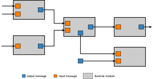
The Basilisk module interface: output messages from one module feed into input messages of the next. Connecting these messages is how a spacecraft simulation is assembled.

The execution model is built around three concepts: Processes, Tasks, and Modules. A SimBaseClass container holds one or more processes, each of which owns one or more tasks, and each task holds a list of modules that are called in order at a specified time step. Every simulation starts the same way:

The time step, which is 2 seconds in the example above, is specified in nanoseconds using the macros.sec2nano() utility. Everything in Basilisk's internal clock runs in nanoseconds, which initially felt unusual, but it turns out it eliminates floating-point precision issues that would accumulate over multi-day mission simulations.

The modules communicate exclusively through typed messages. A module declares one or more output messages, which other modules subscribe to via their input message connections. There is no shared global state and information only flows through explicitly declared message subscriptions. This matters enormously for my project, because when I wrap Basilisk inside a Gymnasium environment, the "observation" that the RL agent receives will be exactly the output of the simpleNav navigation module, and the "action" it outputs will be written directly into the THRArrayOnTimeCmdMsg thruster command message. The message architecture is, conveniently, already the interface I need.

03 The Thruster Example, Taken Apart

The most important script I worked through this week was scenarioOrbitManeuverTH, which simulates a full Hohmann transfer from Low Earth Orbit to Geostationary Orbit using finite thruster burns rather than the instantaneous impulsive delta-v used in earlier simpler examples. This distinction is critical for my project. Prior Basilisk orbit maneuver examples like scenarioOrbitManeuver just add a velocity vector to the spacecraft state at a specific instant, which is convenient but physically unrealistic. For RL-based control, I need the spacecraft to actually fire a thruster for a computed duration, consuming propellant, building up velocity through a force that acts over time, and with an attitude controller that keeps the spacecraft pointed in the correct burn direction throughout. This example does all of that.

The thrusterStateEffector Module

The thruster is modeled via the thrusterStateEffector module, which is the physically correct approach for finite burns. Unlike a simple force vector added externally, the state effector formulation properly couples the thruster dynamics to the spacecraft's equations of motion. The mass changes as propellant is consumed, and this is tracked self-consistently through the integration. Each thruster is defined via the simIncludeThruster.thrusterFactory() utility, which takes a thruster model type, its location in the body frame, its pointing direction, and parameters including maximum thrust, nozzle area, and specific impulse:

The thruster is commanded through the THRArrayOnTimeCmdMsg message, which specifies how long each thruster in the array should fire. The burn duration is calculated analytically before each phase under a constant-mass assumption, which is standard practice for rough planning when the propellant fraction is small:

This constant-mass approximation becomes less accurate as the propellant fraction increases. For the deep-space missions I am targeting, where propellant mass can be a large fraction of total spacecraft mass, I will eventually need to use a proper finite-burn propagation that accounts for continuously changing mass through the rocket equation. Basilisk's thrusterStateEffector already does this integration internally and the approximation is only used here to estimate how long to command the burn. The simulation itself correctly propagates the mass change.

Attitude Control During the Burn

A spacecraft cannot just fire a thruster in an arbitrary direction and it has to be pointed correctly first. This example uses a full attitude control loop to keep the spacecraft aligned with the velocity vector throughout the burn, which is the correct direction for a Hohmann transfer. Five modules work together to make this happen, and understanding each of them is essential because I will need an equivalent attitude-keeping loop in my RL environment to make the commanded thrust go in the right direction.

The velocityPoint module deserves special attention here. It takes the spacecraft's translational navigation state and computes a reference attitude that aligns the spacecraft with the orbit velocity frame. For my RL environment, I will need an equivalent velocity-pointing capability for thrust maneuvers. The attitude control loop runs inside Basilisk; the RL policy only needs to specify when and for how long to fire the thrusters, not how to orient itself during the burn.

The Variable-Timestep Integrator

One subtle but important choice in the example is the use of the svIntegratorRKF45 integrator rather than the default fixed-step RK4. The RKF45 (Runge-Kutta-Fehlberg 4th/5th order) is a variable-step integrator that adapts its step size to maintain a target local truncation error. During the coast phases, where dynamics are smooth, it can take large steps. During and immediately after a burn, when the thrust is changing the trajectory rapidly, it automatically tightens the step size to maintain accuracy.

For deep-space missions with long coast arcs interspersed with short burns, this variable-step capability is necessary for getting numerically accurate results without prohibitive computational cost. I had already flagged computational efficiency as a major challenge and the RKF45 integrator is one of Basilisk's tools for managing this tradeoff.

State Recovery: rv2elem and elem2rv

The orbitalMotion utility module provides the classical orbit element conversions I studied from Schaub and Junkins last week. The two most important functions are orbitalMotion.rv2elem(mu, r, v) and its inverse orbitalMotion.elem2rv(mu, oe). In the example, rv2elem is called after the first burn to compute the current orbital elements and then find the time to apogee, where the second burn will occur. This is a direct illustration of the state representation question I raised last week: the simulation propagates in Cartesian coordinates, but physically meaningful decisions (like "when is apogee?") require the orbital element representation.

The RL agent will need access to this conversion. When constructing the observation vector for the policy network, I plan to augment the raw Cartesian state with the derived orbital elements, as I discussed last week. The orbitalMotion module makes this straightforward because with every step, after calling scSim.ExecuteSimulation(), I can call rv2elem on the current state and append the elements to the observation.

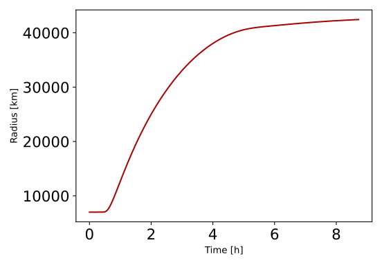
The orbital radius during the Hohmann transfer in scenarioOrbitManeuverTH. The initial flat region at ~7,000 km is LEO; the two burns are visible as the upward ramp during the transfer ellipse; the final plateau near GEO (~42,000 km) is the circularized target orbit.

04 Multi-Body Trajectories and Hyperbolic Arrivals

The thruster example gave me confidence in the core simulation loop, but my project requires more than Earth-orbiting maneuvers. I spent the second half of the week studying two examples that directly address the interplanetary and multi-body dynamics I will need: scenarioPatchedConics and scenarioJupiterArrival.

The scenarioPatchedConics example is particularly instructive because it is the closest existing Basilisk scenario to my eventual problem. It simulates a full Earth-to-Jupiter transfer, beginning with a hyperbolic departure from LEO, proceeding through a heliocentric Hohmann transfer ellipse, and arriving at a Jupiter flyby, all in one continuous simulation. Critically, it does this by running Basilisk's N-body integrator throughout, with Earth, Sun, and Jupiter all contributing to the gravitational acceleration simultaneously. The patched-conics model is used only to design the initial trajectory; the simulation propagates the actual dynamics with all bodies included from the start.

Basilisk always propagates the state in a single inertial frame, but the user changes which body is designated the central body for logging purposes as the spacecraft transitions between gravitational regimes. Early in the simulation, position and velocity are logged relative to Earth. After crossing the Earth's sphere of influence, the central body is switched to the Sun for the heliocentric transfer phase. As the spacecraft approaches Jupiter, the central body switches again. The code manages this by stopping the simulation, adjusting the spacecraft's state vector to account for the offset between reference frames, and restarting with a new logging frame.

The standard approach of always using heliocentric inertial coordinates for the state vector, and only switching to planetocentric coordinates for reward computation near flyby bodies, seems to be what Basilisk supports naturally. The message logged by simpleNav always reports state relative to the current central body, so I will need to be careful about which body is designated central at each phase when reading out the observation for the RL agent.

The scenarioJupiterArrival example covers a hyperbolic capture maneuver. The spacecraft arrives on a hyperbolic approach trajectory, propagates to periapsis, and then fires an impulsive delta-v burn to slow down into a circular parking orbit. This example demonstrated concretely how Basilisk handles hyperbolic orbits. The state initialization uses the same orbital element structure (orbitalMotion.ClassicElements()), with a negative semi-major axis indicating the hyperbolic conic. The simulation time for the first phase (initial position to periapsis) is computed from the hyperbolic time equation:

where $\zeta = \cos^{-1}\!\left(\frac{ea}{a-r}\right)$ is the hyperbolic anomaly analog to the eccentric anomaly on an ellipse. The orbitalMotion module handles these conversions, so I do not need to implement the hyperbolic time equation myself, but understanding it is essential for computing meaningful observation features (like "time to periapsis") for the RL agent during a flyby approach.

There is also a dedicated scenarioFlybySpice example that uses real SPICE ephemeris kernels to drive the spacecraft through Venus, Earth, and Mars flybys with accurate planetary positions. This example additionally shows the velocityPoint module being used to align the spacecraft with the velocity frame during flybys and is the exact same attitude guidance module that the thruster example uses during burns. For my project, this SPICE-driven approach becomes relevant once I need to simulate actual historical mission geometries for validation purposes, though I will start with simplified fixed-planet models to keep the first iteration manageable.

05 The Monte Carlo Machinery

Monte Carlo validation is the primary means by which I will demonstrate that the trained RL policy is actually robust to realistic uncertainties, not just a policy that memorized a specific nominal trajectory. Basilisk has a built-in Monte Carlo framework, and studying it this week showed what kind of validation I should plan for.

The scenarioMonteCarloAttRW example demonstrates the complete MC setup. The entry point is the Controller class from Basilisk.utilities.MonteCarlo. The user specifies the number of runs, the random seeds, and the number of parallel threads. Then dispersions, or the statistical distributions over simulation parameters that will be sampled independently in each run, are defined:

For my trajectory optimization application, the dispersions I care about are directly analogous to those used in Zavoli and Federici (2021): initial state noise (position and velocity errors representing navigation uncertainty), control actuation errors (thrust magnitude and direction errors), and missed thrust events (a run where a planned burn partially or fully fails). The Basilisk MC framework can accommodate all of these through its dispersion API.

One important implementation note from the MC documentation: all simulation objects that will be varied between runs must be attached as attributes of the simulation container (scSim). If a module is only stored in a local Python variable, the MC framework cannot find it to apply the dispersion. This is a subtle but critical requirement that I will need to respect when designing my Gymnasium wrapper. The wrapper class will need to store all Basilisk modules as attributes that the MC framework can reference.

06 Mapping Basilisk to a Gymnasium Environment

Having now worked through Basilisk's architecture and the relevant examples in detail, I can state concretely what the Gymnasium wrapper needs to do. This is the central implementation task of next week, and it is worth being explicit about the design before writing any code.

A Gymnasium environment implements four methods: reset(), step(action), render(), and a definition of the observation and action spaces. The mapping to Basilisk is as follows.

The biggest open question is the granularity of the RL decision step. Each call to step() advances the simulation by some time interval dt_step. If this is set to 2 seconds (the integration timestep), the RL agent makes thousands of decisions per orbit. If it is set to 1 hour, the agent makes coarser decisions but the episode is tractable in terms of total timesteps. The Zavoli and Federici approach used 40 fixed decision points across the entire Earth-Mars transfer, which amounts to roughly one decision every 9 days. I will begin with a similar coarse discretization and refine based on training stability.

07 Looking Ahead

The next two weeks are the most concrete implementation phase of the entire project. Week 4 is for finalizing the MDP formulation of state space, action space, and a preliminary reward function, along with starting the Gymnasium wrapper architecture. Week 5 is for getting the basic wrapper class functional: initialization, state observation, and episode termination logic. The baseline from which I want to depart is a working environment where a random policy can run episodes without crashing, even if it achieves nothing useful. Getting to that baseline, combined with what I learned this week about Basilisk's module structure, is the critical path.

A few specific challenges I am thinking about. The first is the cold start problem of the simulation. Every call to reset() needs to create a fresh simulation object, configure all the modules from scratch, and call InitializeSimulation(). Basilisk does not have a built-in checkpoint-restore mechanism, so there is overhead associated with each episode reset. For RL training with millions of environment steps, this overhead will accumulate. I may need to profile how long InitializeSimulation() takes for different mission configurations and decide whether to accept this cost or find a workaround.

The second challenge is the reference frame consistency issue raised by the patched conics example. During training, episodes will span different mission phases, including Earth departure, heliocentric cruise, flyby approach, and the observation representation needs to be consistent across these phases. I am leaning toward always using heliocentric inertial coordinates for the position and velocity components of the observation, and computing planetocentric elements separately only for reward computation near flyby bodies. This avoids the discontinuities that would arise from switching the primary reference frame mid-episode.

One question I would appreciate feedback on from anyone reading this: for building a Gymnasium-compatible wrapper around a simulation framework like Basilisk, is it better to run the Basilisk simulation in a separate process and communicate with it via inter-process messaging (for robustness and clean separation), or to run it in the same Python process as the RL training loop (for lower latency per step)? My current plan is same-process, but I am wondering whether it may be problematic to reset and re-run many times within the same Python session without memory leaks.