Four Runs, Three Failures,
One Fix

01 Where We Left Off

Welcome back. Last week, the agent finally learned to execute a clean two-burn Hohmann transfer. The v7 model reached the target orbit with under 1.3% SMA error across all evaluation episodes, with two clearly concentrated burns at periapsis and apogee. That was a perliminary answer to the first half of the research question: can an RL agent learn the right orbital maneuver strategy? The second half is more demanding: does the policy hold up when the environment is no longer clean?

Real spacecraft navigate with imperfect components and unmodeled forces. This week I built a five-channel perturbation system to inject all of that into training, then ran four training campaigns to understand what it takes to produce a policy that is both accurate and robust.

02 Five Ways to Break a Spacecraft

The perturbation system follows the framework from Federici et al. (2020), adapted for the Basilisk simulation. The idea is to inject realistic uncertainty into every layer of the spacecraft-environment interface so that the trained policy learns to handle noise as a permanent feature of the world rather than an occasional nuisance.

Channel 1: Observation Noise

Gaussian noise is added to the raw position and velocity measurements before any other computation happens. Everything the agent observes, including the derived semi-major axis, eccentricity, and true anomaly, is computed from those noisy measurements. Position noise is $\sigma = 500$ m and velocity noise is $\sigma = 0.5$ m/s, calibrated to ground-tracking accuracy for low Earth orbit. At a typical orbital radius of 7,000 km, 500 m is about 0.007% of the orbital radius, so it barely affects any single observation but creates enough cumulative uncertainty to matter.

Channel 2: Actuation Magnitude Noise

The commanded burn fraction is multiplied by a factor drawn from $\mathcal{N}(1, \sigma=0.05)$, clipped to $\pm 10\sigma$. A 5% thruster magnitude uncertainty means a commanded full burn might deliver anywhere from 95% to 105% of the nominal thrust. Both the simulation and the fuel accounting use the perturbed value, so the agent cannot rely on its commands being executed exactly.

Channel 3: Actuation Pointing Noise

Even if the thruster fires at exactly the commanded duration, the attitude controller is not perfect. The burn fraction is additionally multiplied by $\cos(\theta_\text{err})$ where $\theta_\text{err} \sim \mathcal{N}(0, 1°)$. At 1° the efficiency loss is under 0.02%, negligible for any single burn. Over 40 steps, and combined with the other channels, the agent experiences a consistent slight underperformance relative to what it commanded.

Channel 4: Dynamics Noise

Before each simulation step, a random inertial force is injected via a dedicated force effector in Basilisk and then zeroed immediately after the step completes. The force magnitude per axis is drawn from $\mathcal{N}(0, m \cdot \sigma_{dv} / \Delta t)$ where $\sigma_{dv} = 1$ m/s, giving each step a random velocity perturbation of roughly 1 m/s per axis. This represents the aggregate of unmodeled higher-order gravity, solar radiation pressure, and atmospheric drag residuals. It is calibrated to be much larger than the real noise level so that training is actively challenging.

Channel 5: Missed Thrust Events (MTEs)

At each decision step, with some probability, the burn command is silently zeroed regardless of what the agent sent. This models a thruster command dropout or a discrete failure. The event counter is capped per episode. I started with a 5% probability (about 2 missed burns per episode expected) and later reduced it to 2% (about 0.8 missed burns per episode), which matches a realistic 99% thruster reliability rate. This change had a much larger effect on training than expected, and I will come back to it.

Channel 6: J2 Gravity

Optionally, the point-mass Earth model is replaced with a degree-2 spherical harmonics model using the GGM03S gravity coefficients. J2 is the dominant perturbation for low Earth orbit, responsible for nodal precession of roughly 1 km per orbit for the orbit altitudes used here. Basilisk downloads the coefficient file automatically on first use and caches it locally.

03 v8: Training Under Perturbations

v8 was the first run with all five perturbation channels active. It used the same PPO hyperparameters as v7 (ent_coef=0.015, clip_range=0.1) but trained in a perturbed environment where the agent never experiences clean physics. After training for 10 million steps across 14 parallel environments, the training curve climbed to a peak reward of roughly 185 and stayed there.

v7, the clean-physics model from last week, peaked at 192 at 8.4 million steps and then collapsed catastrophically at 9.85 million, ending at around 28. The perturbed v8 model not only recovered less than v7 at its peak but held on throughout with no collapse. At the time, the stability looked like a benefit of training under noise. The actual explanation emerged only after looking at v9 and v10.

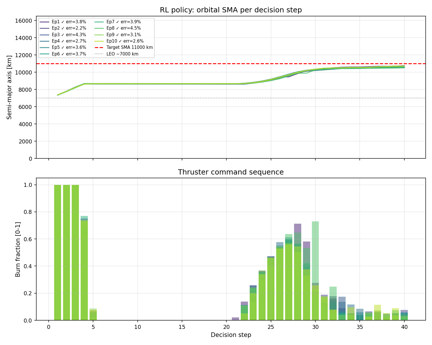
v8 evaluation trajectories under perturbations. All episodes reach the target orbit, but the burn command panel shows energy spread across multiple steps rather than two sharp pulses.

The trajectories tell a more mixed story. v8 reaches the target orbit reliably, but the burn commands are smeared across many steps rather than concentrated at the two Hohmann nodes. Compared to v7's clean two-pulse structure, v8 looks like it is hedging, distributing thrust across a wider window rather than committing to a single decisive burn at each location.

I also built a Monte Carlo evaluation script this week to measure performance statistically rather than just plotting 20 episodes. The script runs N independently-seeded stochastic episodes, reports a success rate with a 95% Wilson confidence interval, and produces histograms of SMA error, fuel use, and reward. Under a 100-run evaluation, v8 shows strong success rates under perturbations, particularly compared to v7 which was never trained to handle noise.

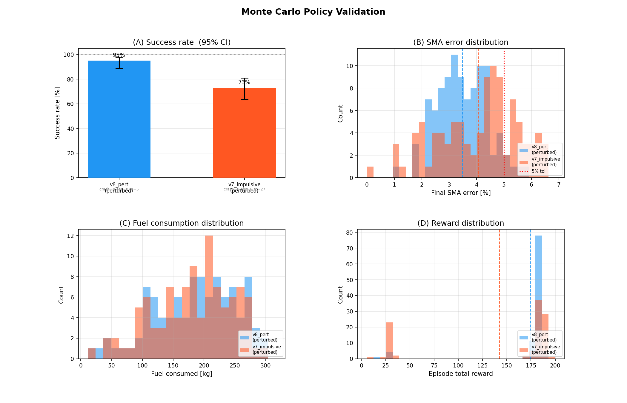
100-run Monte Carlo evaluation comparing v8 (perturbation-trained) against v7 (clean-trained) under live perturbations. Success rate, SMA error distribution, fuel use, and reward distribution.

04 v9 and v10: Two Failures, Two Diagnoses

First, the observation noise fix described above: noise now propagates from raw position and velocity into all derived orbital elements. This is strictly more correct than the previous formulation.

Second, the missed-thrust probability was reduced from 5% to 2%. At 5%, the agent expected roughly 2 missed burns across a 40-step episode. At 2%, it expects 0.8. The rate of 2% corresponds to 99% thruster reliability, which is a reasonable real-world figure. The 5% rate was chosen for training convenience rather than physical accuracy.

v9: The MTE-Entropy Coupling

v9 used the corrected obs noise and 2% MTE, with ent_coef=0.015 carried over from v8. The run peaked at 174 around 2.3 million steps and then collapsed to negative reward in about 50,000 steps, spending the remaining 7.7 million steps producing essentially nothing.

The root cause is a coupling between missed-thrust rate and entropy. In v8, every step had a 5% chance of randomly zeroing the action, which means even a near-deterministic policy experienced substantial reward variance from episode to episode. This variance acts like implicit entropy regularisation, keeping the policy stochastic at the level of training outcomes, supplementing the explicit ent_coef term. With 14 parallel environments and 5% MTE, roughly 87% of episodes experienced at least one action override, making the policy's effective exploration level much higher than ent_coef=0.015 alone would produce.

At 2% MTE, only about 55% of episodes have any missed thrust event. The training environment is roughly 2.5 times less stochastic. The policy converged to a sharp strategy much faster, reaching peak reward at 2.3 million steps instead of v8's 7.2 million, and that fast convergence led immediately to entropy death. Once the policy became too deterministic, small policy updates could not push it out of the local basin, and the basin it settled into turned out not to be the global optimum.

v10: The Constant Learning Rate Problem

The diagnosis of v9 suggested raising ent_coef to compensate for the reduced MTE stochasticity. v10 raised it from 0.015 to 0.025. The training curve rose to around 177 reward, but instead of collapsing, it began oscillating. Over the next 5 million steps, the reward flipped 12 times between the good basin at around 177 and the bad basin at around 25, eventually getting trapped permanently in the bad basin around 7.5 million steps.

This failure mode is different from v9's. v10 found the good basin repeatedly but could not stay there. The reason is that PPO updates the policy by a fixed step size regardless of where in training the policy currently is. At 1 million steps the policy has a lot to learn, and a step size of 3e-4 is appropriate. At 7 million steps the policy is near-optimal, and the same update magnitude is large enough to knock the policy off the narrow reward peak entirely. With ent_coef=0.025 actively trying to spread the action distribution, the combination of a non-decaying learning rate and a high entropy coefficient produced a machine that oscillated the policy in and out of the good basin every 600,000 steps until it eventually lost the path back.

05 The Fix: Learning Rate Annealing

The root cause shared by both v9 and v10 is a learning rate that never decreases. In v9, a constant LR allowed fast convergence to a sharp, brittle policy. In v10, a constant LR applied update steps of equal size at step 7 million (where the policy was near-optimal) as at step 1 million (where the policy had little learned). The fix is linear annealing: both the learning rate and the PPO clip range decay linearly from their initial values to zero over the full training run.

By 7 million steps, the effective learning rate is 9e-4, three times smaller than the value that caused v10's oscillations. Entropy noise of magnitude ent_coef=0.015 can no longer generate gradient steps large enough to cross the basin boundary. The clip range annealing has the same effect on the PPO policy ratio constraint, tightening the allowed policy change as the policy matures.

With LR annealing handling late-training stability, there is no longer a need to push ent_coef up to 0.025 as a substitute. Dropping back to 0.015 produces a sharper action distribution, which means more concentrated burns at the two optimal nodes rather than the diffuse spread-burn strategy that v10's high entropy coefficient enforced.

This is standard practice in deep RL, used in the original OpenAI Atari PPO runs. Without annealing, a near-optimal policy is continuously subjected to destabilising gradient updates, which makes late-training collapse or oscillation nearly inevitable for any environment with a sharp reward landscape.

06 v11: Annealed Training

v11 uses ent_coef=0.015, LR annealing on by default, 2% MTE, physically-consistent observation noise propagation, and all five perturbation channels active. As a result, we end up with v8 but with burns that are more concentrated at the two Hohmann nodes rather than diffused across the episode.

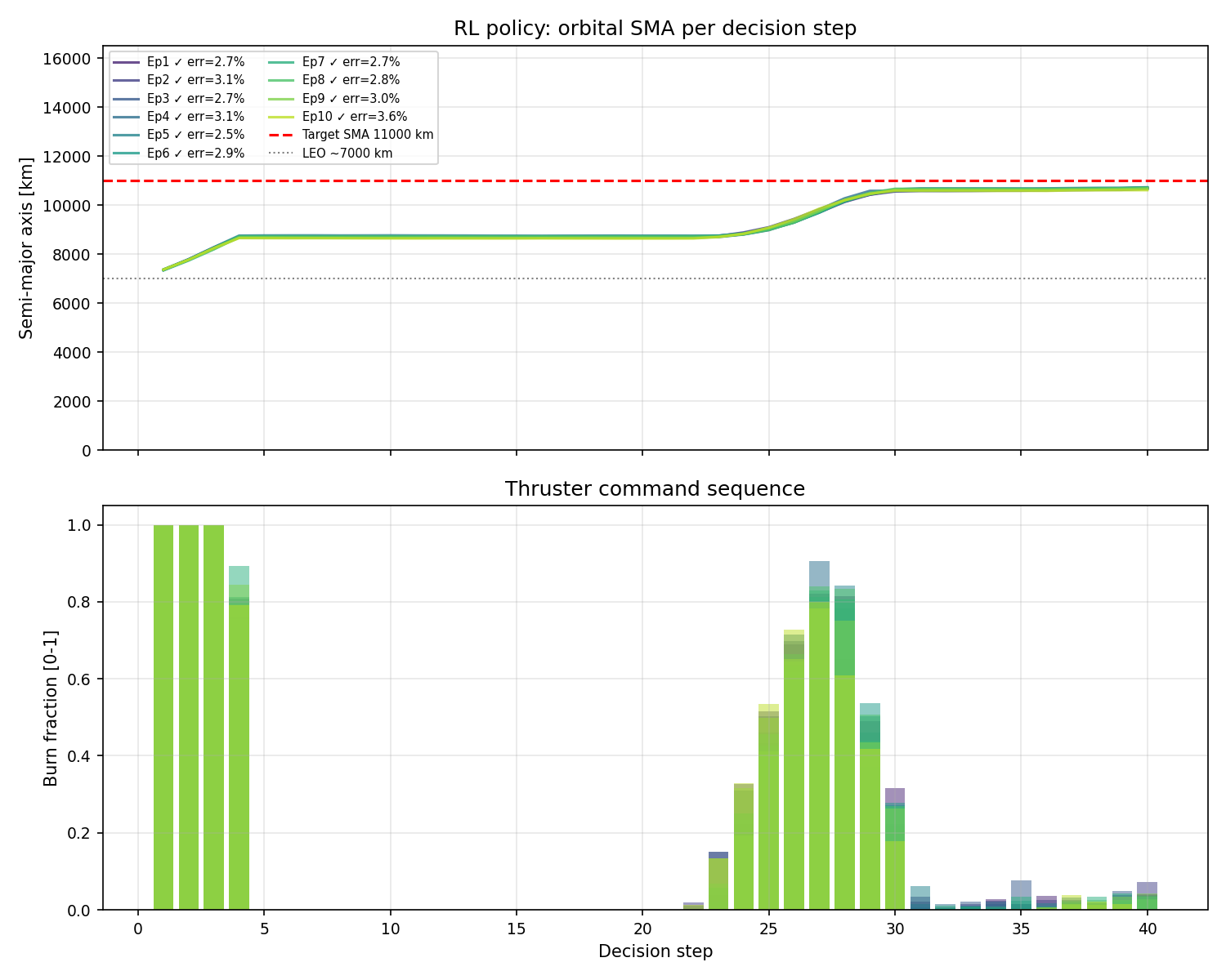
v11 evaluation trajectories under perturbations. The burn command panel shows tighter, more concentrated pulses than v8, closer to the two-burn Hohmann structure that v7 demonstrated in clean physics.

The key question v11 answers is whether a policy can simultaneously be robust to perturbations and execute a clean two-burn strategy. v7 achieved clean burns but on clean physics. v8 achieved robustness but at the cost of a hedged, diffuse burn structure. The combination of LR annealing and realistic 2% MTE gives the agent a training environment that is noisy without over-regularising the action distribution, and the trajectory plots show the tighter burns near the correct orbital locations.

07 What Comes Next

The Hohmann transfer problem for Earth orbit is essentially solved. The agent discovers the correct two-burn strategy, generalises across randomised orbit sizes within the MEO band, and remains robust under realistic sensor noise, thruster uncertainty, and unmodeled forces. There is still room to characterise v11 further through Monte Carlo runs across different noise levels, but the core problem is understood.

The natural next challenge is a longer-range transfer. An Earth-to-Mars Hohmann transfer shares the same mathematical structure with two impulsive burns, one to exit Earth's heliocentric orbit and one to match Mars's, with a coast arc spanning roughly 260 days in between; however, the simulation timescale changes from hours to months and the target is a moving body rather than a fixed orbital altitude.

The question I am most curious about is whether the same reward design, specifically the doubly-quadratic location bonus that teaches the agent to burn at periapsis and apogee, transfers directly to the interplanetary case. In the Earth-orbit setting, periapsis and apogee have fixed geometric meanings relative to the orbit. In the interplanetary case, the departure burn must happen at the right point in Earth's orbit around the Sun, and the arrival burn must happen at the right point in the transfer ellipse, which is determined by the relative positions of Earth and Mars at launch. Whether the reward shaping can guide the agent to discover the correct departure and arrival windows autonomously is the central experiment for next week.